Estimate path coefficients for a DAG.

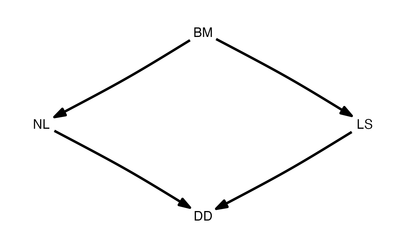
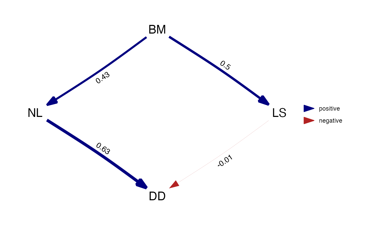
This function will estimate the path coefficients for a DAG, and return them with uncertainty.

Usage

est_DAG(
  DAG,
  data,
  tree,
  model = "lambda",
  method = "logistic_MPLE",
  boot = 0,
  ...
)

Arguments

DAG

A directed acyclic graph, typically created with DAG.

data

A data.frame with data. If you have binary variables, make sure they are either character values or factors!

tree

A phylogenetic tree of class phylo.

model

The evolutionary model used for the regressions on continuous variables. See phylolm::phylolm for options and details. Defaults to Pagel's lambda model

method

The estimation method for the binary models. See phylolm::phyloglm for options and details. Defaults to logistic MPLE.

boot

The number of bootstrap replicates used to estimate confidence intervals.

...

Arguments passed on to phylolm:

lower.bound: optional lower bound for the optimization of the phylogenetic model parameter.

upper.bound: optional upper bound for the optimization of the phylogenetic model parameter.

starting.value: optional starting value for the optimization of the phylogenetic model parameter.

measurement_error: a logical value indicating whether there is measurement error sigma2_error (see Details).

Arguments passed on to phyloglm:

btol: bound on the linear predictor to bound the searching space.

log.alpha.bound: bound for the log of the parameter alpha.

start.beta: starting values for beta coefficients.

start.alpha: starting values for alpha (phylogenetic correlation).

Value

An object of class fitted_DAG, which is a list with the following components:

coef

a matrix of path coefficients, with predictors in the rows and responses in the columns. Absent paths are 0.

se

a matrix of standard errors of the coefficients.

lower, upper

matrices with the bounds of the bootstrapped confidence intervals, only present if boot was larger than 0.

binary

a named logical vector marking which variables were modelled as binary.

Details

Continuous variables are standardized before fitting, that is, centered and divided by their standard deviation, while binary variables are left as they are. In the two usual cases this means the coefficients can be compared with each other directly:

• When every variable is continuous, each coefficient is the change in the outcome, in standard deviations, for an increase of one standard deviation in the predictor. These are standardized regression coefficients, as reported by von Hardenberg & Gonzalez-Voyer.

• When every variable is binary, each coefficient is the log odds ratio for the outcome between the two levels of the predictor. A level to level contrast is a natural unit that every binary variable has, so these are comparable too.

When a model contains binary and continuous variables, its coefficients can no longer be compared with one another, for two separate reasons. Paths into a binary variable are log odds ratios while paths into a continuous variable are standardized regression coefficients, which are different units entirely. And a binary predictor contributes a contrast between its two levels, which for a variable where a proportion p of species has one of the levels amounts to 1 / sqrt(p * (1 - p)) standard deviations. That is always more than two, so the coefficients of binary predictors are inflated relative to those of continuous predictors in the same model.

Examples

  d <- DAG(LS ~ BM, NL ~ BM, DD ~ NL + LS)
  plot(d)

  d_fitted <- est_DAG(d, rhino, rhino_tree, 'lambda')
  plot(d_fitted)